Optimizers, Part 1
Happy New Year! This is going to was supposed to be a long
one, so sit back and grab a chocolate (and preferably view this on your laptop)
Some optimization algorithms. Click on a colour in the legend to hide/show it
Table of Contents
Introduction
Most supervised learning tasks involve optimizing a loss function, in order to fit the model to the given training data. Of these, the most common is neural network training: neural networks have millions (even billions) of parameters which need to be tuned so that the model can predict the right outputs.
Obtaining closed form solutions to neural network problems is more often than not intractable, and so we perform this optimization algorithmically and numerically. The main things we look for in an algorithm that optimizes the loss function are:
It should converge: Sounds like a no-brainer, but the algorithm should be able to decide when and where to stop, and to ensure that the location at which it stops is a local minima.
It should converge quickly: The algorithm should take as few steps as possible to converge, as every step requires a parameter update, and updating millions (if not billions) of parameters is inefficient. Therefore, it should take the optimal steps at every point.
It should be able to deal with ambiguity: Loosely worded, the algorithm would not have the exact value of the gradient: all the algorithms described use a batch of samples to obtain an estimate of the gradient, and the expected value of the gradient obtained should equal the gradient of the function at this point. The algorithm should be able to converge to a local minima even if it obtains incorrect gradients at some steps in the process.
Do solutions even exist?
We can’t really go further without knowing what the loss landscape looks like: do solutions even exist? How do we visualize a high-dimensional loss landscape?
A few observations about the loss landscape of a neural network from Goodfellow are:
As dimensionality of the latent space increases, the probability a critical point is a local minima decreases. The curvature of a point is given by the eigenvalues of the hessian: if all the eigenvalues are positive, the point is a local minima (and the hessian is positive semi-definite), and the opposite for a local maxima. If we consider a random function, choosing the sign of the eigenvalue is akin to tossing a coin. Therefore, in n-dimensional space, if we toss n coins to determine these signs, the probability that all of them turn up positive is very low. Therefore, high- dimensional space has more saddle points than local minima/maxima
There are several equally good local minima: because of scale invariance, if you scale the inputs to a layer down by 10 and multiply the outputs by 10, then you get the same resultant network. Also, if you switch the position of two neurons in a layer with each other while maintaining the connections, you get the same network. These two similarities result in a large number of similar optima, reaching any one of which will optimize the entire network.
Both of these are in our favour, and show us that reaching a local minima in high-dimensional space should be sufficient to fit the network. We’ll now take a look at some algorithms which do this.
As for visualizing the loss landscape, this is significantly trickier to do. This work by Goldstein et al does a good job of it, but visualizing and comparing the paths taken by optimization algorithms on this landscape is very difficult: because what we’re seeing is a projection onto two dimensions, the direction taken by the path need not correspond to the direction of maximum descent. This repository by Logan Yang had a good implementation of this paper, along with traces of the paths taken by various optimization algorithms showing why we can’t use this to qualitatively compare different optimization algorithms with each other
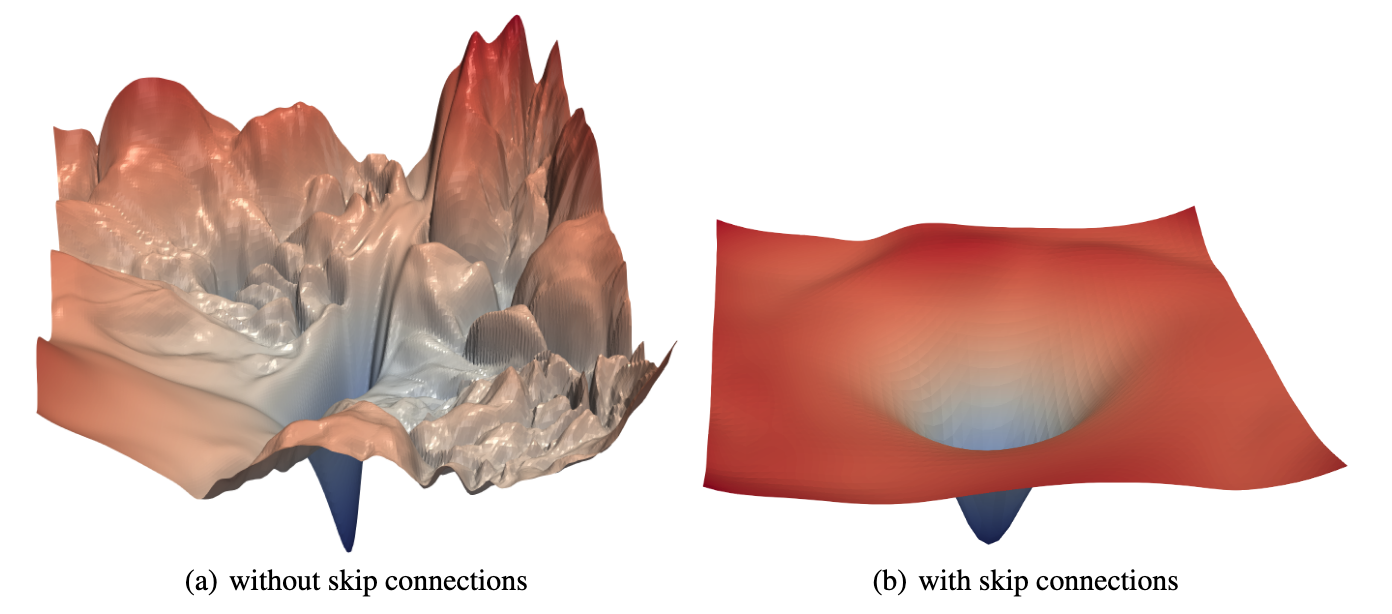
The loss landscape of ResNet-56 (source: Goldstein et al)
How this guide is structured
While most deep learning problems use a super high-dimensional loss function, for the purposes of this guide we’ll use a simple 2-D loss function which is a linear combination of gaussians of the following form $$\begin{gather} f(x, y) = se^{-(ax+by+c)^2} \\ \mathcal{L} = \sum_{i=1}^{n} f_i(x, y) \end{gather}$$
The good thing about gaussians is that they’re easy to differentiate $$\begin{align} \frac{\partial f}{\partial x} &= -2a(ax+by+c)f(x,y) \\ \frac{\partial f}{\partial y} &= -2b(ax+by+c)f(x,y) \\ \frac{\partial^2 f}{\partial x^2} &= -2a^2(1 - 2(ax+by+c)^2)f(x,y) \\ \frac{\partial^2 f}{\partial x \partial y} &= -2ab(1 - 2(ax+by+c)^2)f(x,y) \\ \frac{\partial^2 f}{\partial y^2} &= -2b^2(1 - 2(ax+by+c)^2)f(x,y) \end{align}$$
so all the methods can use the exact gradient/hessian of the loss function rather than a stochastic one. This is kind of cheating, but since this is a science experiment, let’s run with it. about this loss func
$s, a, b, c$ are generated uniform randomly from a suitable range, and I played
around manually with this till I got a loss function that looked funky enough
for my needs. We finally use the following loss function, and it’s been
exported to the file func.dill if you want to load it in (use dill to load it,
as there were some errors serializing it via pickle)
The convergence criterion that’s used for all optimizers is when the gradient norm is less than 0.05, and all the optimizers are limited to take atmost 1000 steps.
The plots are made in Bokeh/Plotly and are interactive (if you haven’t already played with the plot we generated in the start). I’ve done my best to be inspired by Distill, most notably Gabriel Goh’s beautiful, interactive article on momentum.
Gradient Descent Optimizers
Gradient Descent optimizers converge to a local minimum by simply following the gradient: there’s no adaptiveness here, and it’s akin to feeling the area around your feet and just taking a small step in the steepest direction, and repeating that till you get to the minima. There are a few tricks here and we take hints from Physics to speed up the convergence, but most of the algorithm relies on the gradient, and the speed with which we’re already going.
Stochastic Gradient Descent
SGD is probably the first optimization algorithm one thinks of. It’s deceptively simple: Look around and take a step in the direction where the gradient decreases the most. Once you’ve taken the step, Stop, look around again, and repeat until you’re at the minima (the gradient is sufficiently small or you come back to a point you’ve visited).
Th S in SGD comes from the fact that the gradient that the algorithm obtains in practice is not perfect: it’s an approximation of the actual gradient of the loss function, based on the batch of examples that are sampled. However, this approximates the gradient reasonably well, and in the long run, the expected path taken by this algorithm comes out to be the same as the path taken when we can perfectly obtain the gradient.
The update rule for SGD is fairly simple:
$$\begin{align} \theta_{t+1} &\leftarrow \theta_{t} - \epsilon g(\theta_{t}) \end{align}$$
Combining this with a convergence criterion gives us the algorithm (implemented in python here)
def SGD(L, G, p0, eps=5e-2):
    p = p0
    g = np.inf
    while norm(g) > 5e-2:
        g = G(p)
        p = p - eps*g
SGD with Momentum
While SGD is simple, it is slow to converge, taking several more steps than required. This is because we come to a stop once we take a step, and the size of the next step is solely determined by the gradient at that point. This means that if we’re in a long stretch where the gradient is small, we can only descend at the speed $\epsilon g$, even though we know that the stretch is reasonably long. This slows down our algorithm and makes it take a longer time to converge.
Momentum counters this by providing some inertia to the process. Intuitively, if SGD is a person stopping and taking a step in the direction of maximum descent, momentum is equivalent to throwing a ball down the incline of a given mass and seeing where it settles. If you take a look at the path momentum follows in the introduction plot, you can see that it doesn’t immediately stop when it comes to a point with a zero (or very small) gradient; instead, it oscillates until it loses all it’s velocity.
How do we simulate adding ‘mass’ to the update steps? We claim that the ball moves at a velocity $v$, and model $v$ as an exponential moving average of the current velocity and the gradient at the current point. The update equations are as follows:
$$\begin{align} v_{t+1} &\leftarrow \alpha v_{t} - \epsilon g(\theta_{t}) \\ \theta_{t+1} &\leftarrow \theta_{t} + v_{t+1} \end{align}$$
What’s the maximum velocity we can move at? If all the gradients are in the same direction for an infinite (practically a very large) period of time, then this velocity is equal to
$$v_{\text{max}} = \frac{\epsilon g}{1-\alpha}$$
This can be derived by expanding out the recurrence in the update step, to obtain an infinite GP. This GP converges when $\alpha < 1$ to $1/(1-\alpha)$. We can think of $1-\alpha$ as the ‘mass’ of the ball: the smaller this quantity is, the faster the ball will move.
Generally (and in this simulation as well), $\alpha = 0.9$, so $1-\alpha = 0.1$. This means that we can move atmost ten times faster than the step size at a point, and this is what causes momentum to converge faster!
def SGD_momentum(L, G, p0, v0=0, eps=5e-2, a=0.9):
    p = p0
    v = v0
    g = np.inf
    while norm(g) > 5e-2:
        g = G(p)
        v = a*v - eps*g
        p = p + v
What do these gradient updates look like in practice? For starters, all changes in the direction of the path are caused due to changes in the gradient. Where the path takes a turn, the gradient is normal or antiparallel to the current velocity, and at places where the path is straight, both the gradient and the velocity are parallel. We can draw out the update vectors at two points in the path above to see how this works.
SGD with Nesterov Momentum
If you’ve seen the path that momentum takes, there is one issue: Momentum doesn’t stop very soon. It’s easy to get the ball rolling, but harder to stop it. This happens because the gradient that’s added to the path is the gradient at the current point, not the gradient at the point at which we would have been, if we took the step. In a continuous, real-world scenario, this difference is infinitesimal, but in a numerical scenario, it becomes significant if our step size is not small enough. This is also not an issue if our gradients at consecutive points are similar, but becomes an issue if we ‘jump’ across a local minima: momentum would push us even further forward, because the gradient at the current point is downward.
This ‘bug’ was discovered by Nesterov, and the fix was to compute the gradient at $\theta_{t} + \alpha v_{t}$ (the position we will be at, if the gradient is zero) rather than at $\theta_{t}$ (our current position). This ‘pulls’ the gradient back if we jump across a minima
The implementation and update are quite similar, with just a minor update to the gradient calculation.
$$\begin{align} v_{t+1} &\leftarrow \alpha v_{t} - \epsilon g(\theta_{t} + \alpha v_{t}) \\ \theta_{t+1} &\leftarrow \theta_{t} + v_{t+1} \end{align}$$
def SGD_nesterov(L, G, p0, v0=0, eps=1e-2, a=0.9):
    p = p0
    v = v0
    g = np.inf
    while norm(g) > 5e-2:
        g = G(p + a*v)
        v = a*v - eps*g
        p = p + v
Putting it all together
Here’s an interactive demo, showing the paths taken by SGD, SGD with Momentum and SGD with Nesterov Updates. The arrows have the same colour scheme as before, and show the directions in which the path is pulled (their sum is the next resultant step). Playing around with this should give you an idea of how these algorithms update themselves
Even though there are a large number of new algorithms for optimization, SGD with Nesterov momentum (along with Adam) remains the algorithm of choice for training very large neural networks: it’s stable, explainable and converges nicely.
References and Footnotes
- Goh, “Why Momentum Really Works”, Distill, 2017. http://doi.org/10.23915/distill.00006
- Goodfellow, Ian, Bengio, Yoshua and Courville, Aaron. Deep Learning. : MIT Press, 2016.
- Melville, James. Nesterov Accelerated Gradient and Momentum. https://jlmelville.github.io/mize/nesterov.html
This was supposed to also feature adaptive optimizers (AMSGrad, RMSProp, Adam
and friends), but due to CCIC happening in the last week of December, I didn’t
get the time to do this properly, and the second semester starts in a
couple days tomorrow, so hard deadline :/ I’ll try to get part 2 out
as soon as possible, but it might be a while. In the meantime, exploring the
source might help for the impatient.
For the complete code, and to play around and implement your own optimizers, check out the repository here
